When asking the question, “What leads to success at the Olympics?”, economic factors may not immediately jump to mind. However, not only is this a big indicative factor to individual countries success, but plays a huge role overall in the game of winning the Olympics. A higher economic output leads to greater potential investment in sports and training facilities for athletes. Potential being the key word here, as of course its up to each country how they allocate their resources. In this analysis we are going to take a deep dive into this question of how big of an impact Economic factors play in the grand spectacle that is the Olympics.
Code
library(tidyverse)library(DT)library(janitor)library(FSA)library(car)library(lme4)library(MuMIn)library(MASS)library(plotly)library(shiny)options(warn=-1)economy <-read_csv("Global Economy Indicators.csv")economy <- economy |>clean_names()economy <- economy |>mutate(per_capita_gdp = gross_domestic_product_gdp/population)medals <-read_csv("olympics/Olympic_Medal_Tally_History.csv")#Filter for relevant economic datamedals <-filter(medals, year >=1970)#Filter for only Olympic yearseconomy <-filter(economy, year >=1972& year %%2==0)#Weighted medal total, Gold = 3, Silver = 2, Bronze = 1medals <- medals |>mutate(weighted_total = gold*3+ silver *2+ bronze)renamed <- economy |>mutate(country =ifelse(country =="Czechoslovakia (Former)", "Czechoslovakia",ifelse(country =="D.P.R. of Korea", "Democratic People's Republic of Korea",ifelse(country =="Ethiopia (Former)", "Ethiopia",ifelse(country =="China, Hong Kong SAR", "Hong Kong, China",ifelse(country =="Iran (Islamic Republic of)", "Islamic Republic of Iran",ifelse(country =="Saudi Arabia", "Kingdom of Saudi Arabia",ifelse(country =="Former Netherlands Antilles", "Netherlands Antilles",ifelse(country =="China", "People's Republic of China",ifelse(country =="USSR (Former)", "Soviet Union",ifelse(country =="USSR (Former)", "Soviet Union",ifelse(country =="Bahamas", "The Bahamas",ifelse(country =="United Kingdom", "Great Britain",ifelse(country =="Viet nam", "Vietnam",country) ))))))) ) ) ) )))merged <-merge(renamed, medals, by =c("country", "year"))
Datasets
To help answer this question I merged economic indicators of each country by year to our overarching olympic dataset. This isn’t a perfect merge as some Olympic teams dont exactly match their political entities but this should give us a pretty good idea. We can take a quick look at the working dataset which should give us an idea of what we might find when we dive deeper.
To no surprise the United States and the Soviet Union consistently top the list, which were both economic powerhouses in their respective Olympics. This might also say something to the effect of the emphasis each country placed on doing well in the Olympics especially during the Cold War. Regardless its important to note that each year has its own unique slate of events and overall global economic output. To help address this, instead of analyzing based off of raw numbers, I am utilizing a ranked approach. So for each Olympic event countries will be ranked on both GDP output, population and medal output. I.e., the top medal earner for an Olympic event will be ranked 1 and the top GDP producer will be ranked 1 for that metric respectively.
Why GDP?
I think its important to at least go over why GDP was selected as the primary metric. Along with population which is heavily correlated to GDP output (more people leads to on average more economic production), it helps capture the overall economic strength of a country in a simple metric. As opposed to GDP per Capita which normalizes GDP based on population, this better captures the economic might that larger countries generally have. It also helps negate the factor that while China has a compartively low GDP per Capita it still out produces every country now other the the United States. Conversely while a country like Luxembourg has one of the highest GDP per Capitas, it is a tiny country with nowhere near the resources of a bigger economy like Germany for example. GDP correctly measures the size of a countries economy which is what were primarily concerned with here.
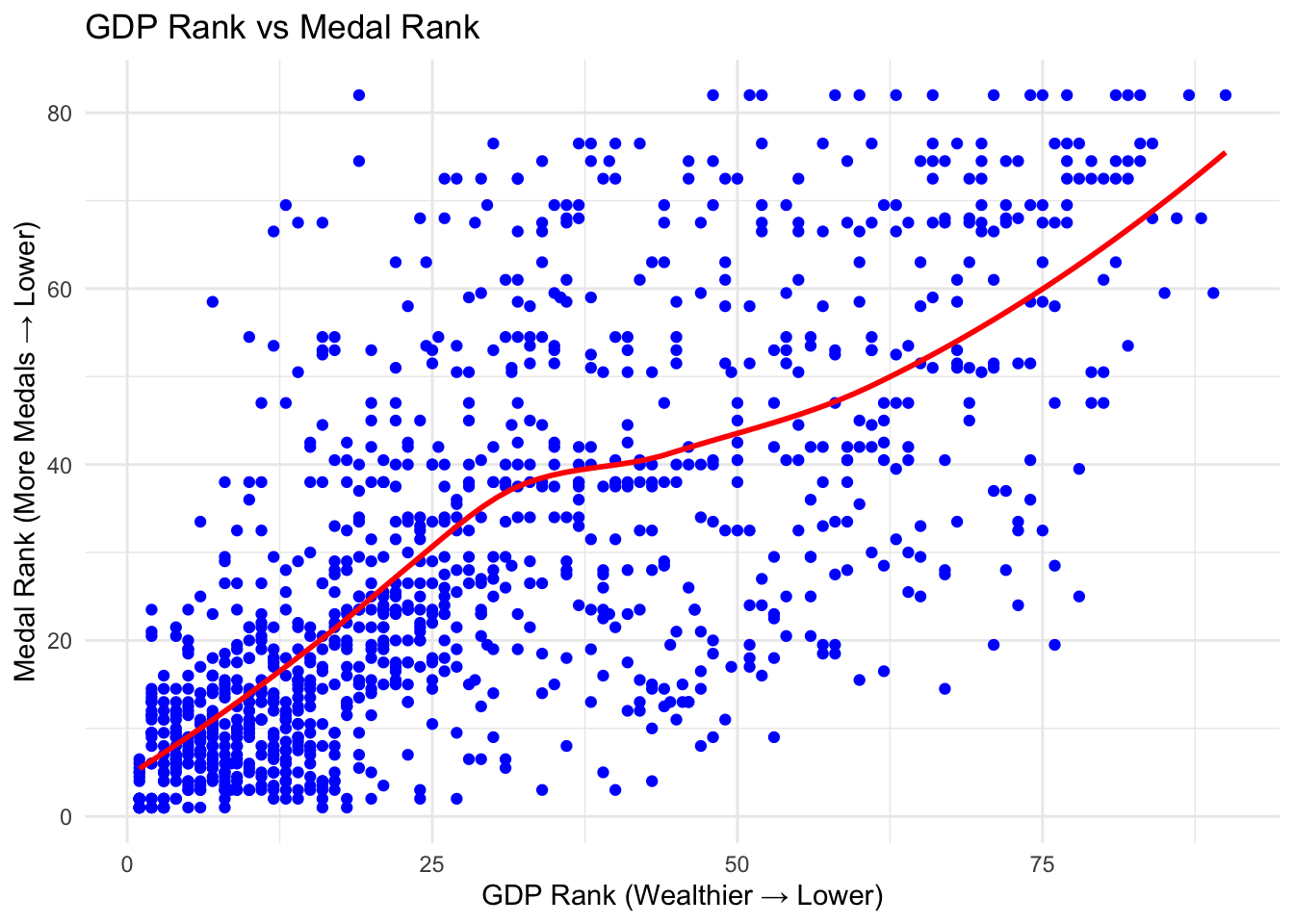
When comparing the GDP ranks with the medal ranks, the general assumption does seem to fit. Higher GDP producers tend to dominate the top ranks of medal earners. The spread is more consistent near the first quadrant of data, i.e. top 25 medal earners and top 25 GDP producers and then spreads out more as the ranks get higher. This can be illustrated in the graphic above, when fitting the data to a LOESS regression, there is a pretty strong linear relationship at the start that gets less strong as the ranks decrease.
Code
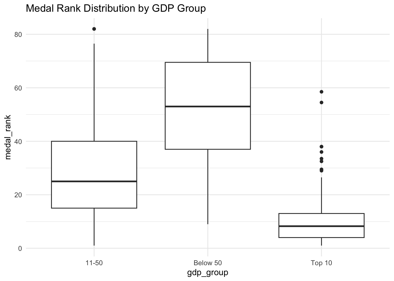
ranking <- ranking |>mutate(gdp_group =case_when( gdp_rank <=10~"Top 10", gdp_rank <=50& gdp_rank >10~"11-50",TRUE~"Below 50" ))ggplot(ranking, aes(x=gdp_group, y=medal_rank)) +geom_boxplot() +labs(title="Medal Rank Distribution by GDP Group") +theme_minimal()
When conducting a group analysis, the effect of GDP is perhaps more evident. Separating countries into three groups, Top 10 in GDP, the next 40 and the bottom producers, the general ranges fall very in line with their medal ranks. Of course there are outliers and exceptions but this boxplot does help visualize the heavy relation between top economic countries and success at the Olympics.
Code
# Define the UI for the applicationui <-fluidPage(titlePanel("Interactive GDP Rank vs Medal Rank"),sidebarLayout(sidebarPanel(# Dropdown for selecting countryselectInput("country", "Select Country", choices =c("All Countries", unique(ranking$country)), selected ="All Countries"),# Slider for selecting the yearselectInput("edition", "Select Olympic Edition", choices =c("All Editions", sort(unique(ranking$edition))), selected ="All Editions") ),mainPanel(plotlyOutput("interactive_plot") ) ))# Define the server logic for the applicationserver <-function(input, output) {# Reactive expression to filter the data based on user input filtered_data <-reactive({if (input$country =="All Countries") { country_data <- ranking } else { country_data <- ranking |>filter(country == input$country) }# If "All Editions" is selected, use all editions; otherwise, filter by selected editionif (input$edition =="All Editions") { filtered <- country_data } else { filtered <- country_data |>filter(edition == input$edition) }return(filtered) })# Generate the plot output$interactive_plot <-renderPlotly({ plot_data <-filtered_data()# Create the plot with ggplot p <-ggplot(plot_data, aes(x = gdp_rank, y = medal_rank)) +geom_point(color ="blue", aes(text =paste("Country:", country, "<br>GDP Rank:", gdp_rank, "<br>Medal Rank:", medal_rank))) +geom_smooth(method ="loess", color ="red", se =FALSE) +labs(title ="GDP Rank vs Medal Rank",x ="GDP Rank (Wealthier → Lower)",y ="Medal Rank (More Medals → Lower)") +theme_minimal()# Convert to plotly for interactivityggplotly(p, tooltip ="text") })}# Run the applicationshinyApp(ui = ui, server = server)
With this interactive graph you can dive deeper into the specific country outputs and how the trends have differed per competition. Feel free to play around and see how the relation progresses over time and how some countries are unique outliers.
Population
The other metric I considered is countrys total population. Of course this should be directly correlated to a countrys GDP, as a higher population leads to more potential yield in the economy although its not always one to one. Logically one might think as a population is higher the chances of producing olympic athletes must also be higher with a larger pool of candidates.
Code
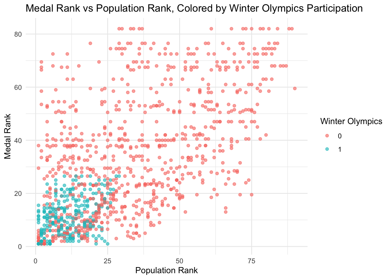
ranking <- ranking |>mutate(winter =ifelse(grepl("Summer", edition), 0, 1))ggplot(ranking, aes(x = pop_rank, y = medal_rank, color =factor(winter))) +geom_point(alpha =0.6) +labs(title ="Medal Rank vs Population Rank, Colored by Winter Olympics Participation",x ="Population Rank", y ="Medal Rank", color ="Winter Olympics") +theme_minimal()
As can be seen in the data, the relationship isnt as strong but exhibits a very similar pattern to GDP. This just further highlights the impact of raw economic output by country has on the Olympics. It is interesting to note that far fewer countries tend to participate in the Winter editions. The winter editions also vary wildly within their smaller sections, implying the higher cost of entry inherent of winter sports negates the GDP factor to some degree albeit it is still present.
Country Factor + Modeling
Ultimately what ends up being the biggest factor that might cause a county to under perform or over perform their raw GDP is their unique characteristics inherent. of each country. Not all countries value sports or the Olympics the same which may cause some countries to push above or below their weight.
Code
model_mixed <-lmer(medal_rank ~poly(gdp_rank, 2) +poly(pop_rank, 2) + winter + (1| country), data = ranking)random_intercepts <-ranef(model_mixed)$countryranking$predicted_medal_rank <-predict(model_mixed, newdata = ranking)ranking$adjusted_medal_rank <- ranking$predicted_medal_rank + random_intercepts[ranking$country, ]ranking$diff_medal_rank <- ranking$adjusted_medal_rank - ranking$predicted_medal_rankagg_data <- ranking |>group_by(country) |>summarise(mean_diff_medal_rank =mean(diff_medal_rank, na.rm =TRUE)) |>ungroup() p <-ggplot(agg_data, aes(x =reorder(country, mean_diff_medal_rank), y = mean_diff_medal_rank)) +geom_bar(stat ="identity", aes(text =paste("Country:", country, "<br>Mean Difference:", round(mean_diff_medal_rank, 2))), width =0.7, fill =ifelse(agg_data$mean_diff_medal_rank >0, "blue", "red")) +coord_flip() +scale_y_continuous(expand =expansion(mult =c(0, 0.05))) +# Adjust y-axis paddinglabs(title ="Mean Effect of Random Intercepts on Medal Rank by Country",x ="Country",y ="Mean Difference in Predicted Medal Rank" ) +theme_minimal()interactive_plot <-ggplotly(p, tooltip ="text") |>layout(width =800, height =1400 )interactive_plot
To capture this effect, a mixed effect model was run to assess the effects certain countries had on their olympic performances. If you explore the graph above you will see the countries in blue with a positive difference on average underperform based on their GDP. While countries in the red tend to overperform their GDP. In mixed-effects models, random intercepts represent the variation in the response variable (e.g., medal_rank) that is attributed to differences between the groups or levels of the random factor (e.g., country in your model). They capture how much each group (in this case, each country) deviates from the global average (the overall fixed effect) in the intercept.
When we judge the model, we see that the Marginal R squared is .49 inidcating a strong relationship between our indicators (population, GDP, and winter vs no winter olympics). However when conditioning on the specific country the R squared is .845 which is very high. This tells us that country specific factors plays a significant role in determining Olympic Success. For example a country like Saudi Arabia significantly under performs its GDP, which can be explained to a lack of investment in sports in that country versus other things like religion. On the other end New Zealand significantly outperforms its GDP indicating the opposite, a high importance is places on sports and athleticism in that country.
Conclusion
Throughout this analysis we have dug into the question of does money buy medals? Well in some cases the answer is yes. More affluent countries perform by in large far better then poorer countries. Now that doesn’t mean its citizens are well off at all, we are just measuring based on raw GDP which is no indication of quality of life or GDP per capita. Luxembourg while top in GDP per capita is not a significant contributor in the Olympics. We are really just analyzing the size of the economy versus how many medals that country earns. Due to higher populations and more ability to invest in athletics those countries do perform better however there are some outliers. Winter Olympics especially, which requires a significant investment to compete in, evens the playing field more and lower GDP countries. comparatively like Austria and Norway are able to shine. When it comes down to it, Economy alone while an indicator, can not predict Olympic success alone. There are clearly unique factors per country that determines its success or lack thereof. After all if you have alot of money but choose to fuel it all towards National Defense, it probably wont lead to a thriving internal sports culture.